Running along the graph using Neo4J Spatial and Gephi
When I started running some years ago, I bought a Garmin Forerunner 405. It’s a nifty little device that tracks GPS coordinates while you are running. After a run, the device can be synchronized by uploading your data to the Garmin Connect website. Based upon the tracked time and GPS coordinates, the Garmin Connect website provides you with a detailed overview of your run, including distance, average pace, elevation loss/gain and lap splits. It also visualizes your run, by overlaying the tracked course on Bing and/or Google maps. Pretty cool! One of my last runs can be found here.
Apart from simple aggregations such as total distance and average speed, the Garmin Connect website provides little or no support to gain deeper insights in all of my runs. As I often run the same course, it would be interesting to calculate my average pace at specific locations. When combining the data of all of my courses, I could deduct frequently encountered locations. Finally, could there be a correlation between my average pace and my distance from home? In order to come up with answers to these questions, I will import my running data into a Neo4J Spatial datastore. Neo4J Spatial extends the Neo4J Graph Database with the necessary tools and utilities to store and query spatial data in your graph models. For visualizing my running data, I will make use of Gephi, an open-source visualization and manipulation tool that allows users to interactively browse and explore graphs.
1. Extracting GPX data
The Garmin Connect website allows to download running data through various formats, including KML, TCX and GPX. GPX (the GPS Exchange Format) is a light-weight XML data format that is used for interchanging GPS data (waypoints, routes, and tracks) between applications and web services. Below, you can find a GPX extract enumerating several tracked points. Each of these points contains the GPS location, the elevation and the corresponding timestamp.
Based upon this data, one is able to calculate various metrics, including pace. For this, we will use GPSdings, a Java library that provides the required functionality to extract and analyze GPX data. We start by reading in a GPX file. Afterwards, we analyze the content using the GPSdings TrackAnalyzer which, amongst other metrics, calculates the pace for each point that was tracked during a run. The information we need is stored in the first segment of the first track.
2. Importing GPS data in Neo4J Spatial
Neo4J Spatial is build on top of Neo4J and provides support for spatial data. Once your data is stored, spatial operations can be executed, which for instance allow to search for data within specified regions or within a specified distance of a particular point of interest. We start by setting up a Neo4J EmbeddedGraphDatabase. We then wrap it as a SpatialDatabaseService, which allows us to create an EditableLayer. EditableLayer is Neo4J’s main abstraction, which is used to define a collection of geometries. Each layer needs to be initialized with a specific GeometryEncoder, which acts a kind of adapter to map from the graph to the geometries and vice versa. In our case, we will employ the SimplePointEncoder.
Adding spatial data to the running layer is very easy. We start by creating a Coordinate for each point that is parsed by GPSdings. Next, we add this new coordinate to the running layer. This operation returns a SpatialDatabaseRecord which, under the hood, is just a regular Neo4J node. Hence, we can add any property we want to this node. In our case, we will add two properties. One property, named speed, indicating the (average) pace. One property, named occurrences, indicating the number of times this particular coordinate was encountered in the overall data set. Once the new coordinate is created, we connect the previous node with the newly created node through the NEXT relationship type. Hence, our graph is an enumeration of the encountered coordinates, interlinked through NEXT edges.
In case a coordinate is encountered multiple times, we recalculate the average speed and increment the number of encounters.
Unfortunately, chances are low to encounter an already existing coordinate, as coordinates in a GPX file have a 15-digit precision right of the decimal point. Instead of trying to round these coordinates ourselves, we will use the Neo4J Spatial querying API. A simple nearest neighbor-search limited to 20 meters allows us to find matching coordinates. (I choose 20 meters, as 20 is a little above the average distance between two coordinates). In case we find a coordinate within this 20-meter range, we will reuse it. Otherwise, we just create a new coordinate. The full algorithm for importing multiple GPX datasets can be found below.
3. Visualizing running data
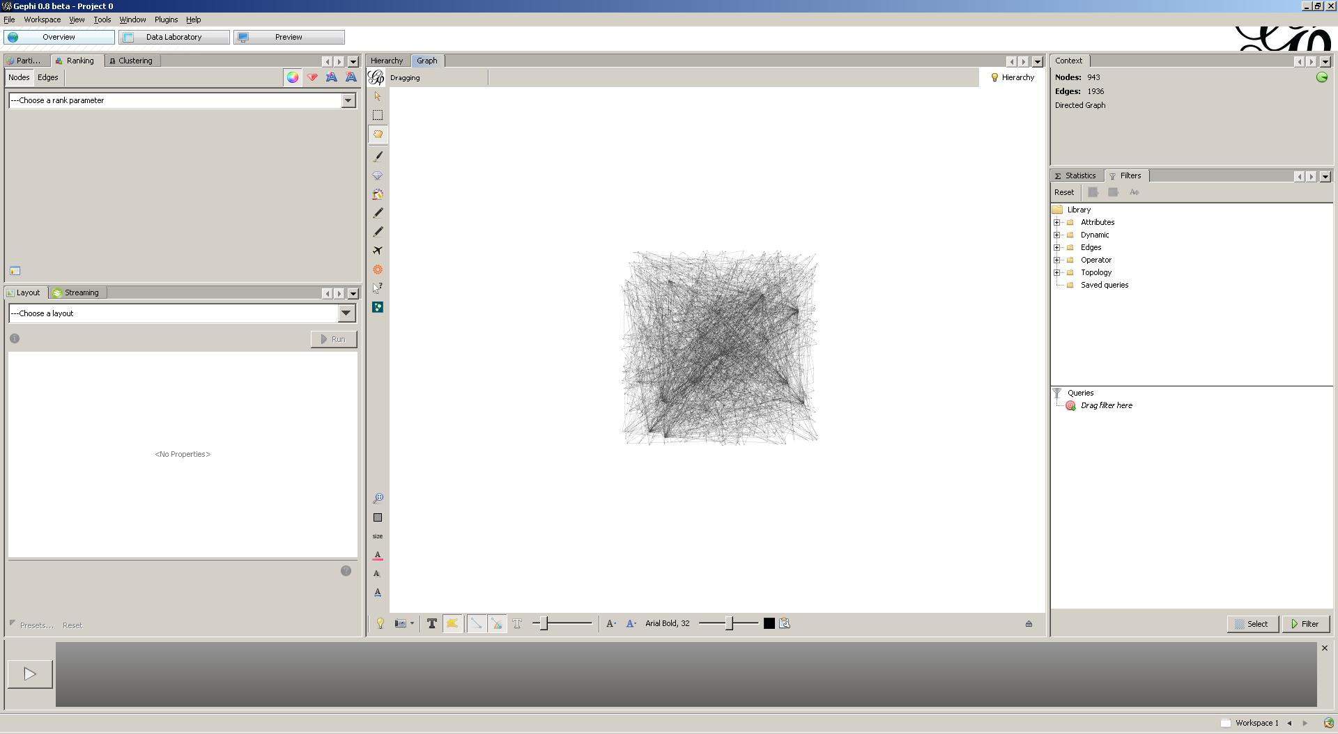
By using the Neo4J Spatial querying API, we are able to retrieve the set of coordinates that satisfy a particular condition. However, coordinates are somewhat abstract to interpret. Instead, we will use the excellent Gephi Graph visualization and exploration tool. By installing the Gephi Neo4J plugin, we are able to load and explore graphs that are stored in a Neo4J (Spatial) datastore. Let’s start by importing our dataset in Gephi.
The displayed graph contains other types of nodes and edges (i.e. Layer and RTree index information), in addition to the coordinates and NEXT edges that we added ourselves. Let’s get rid of those by filtering our graph on the NEXT relationship-type.
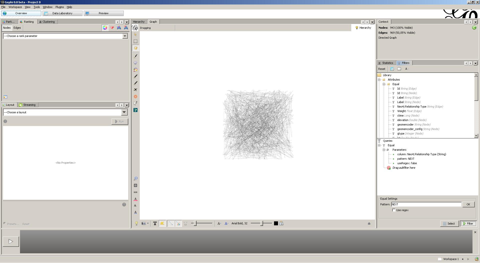
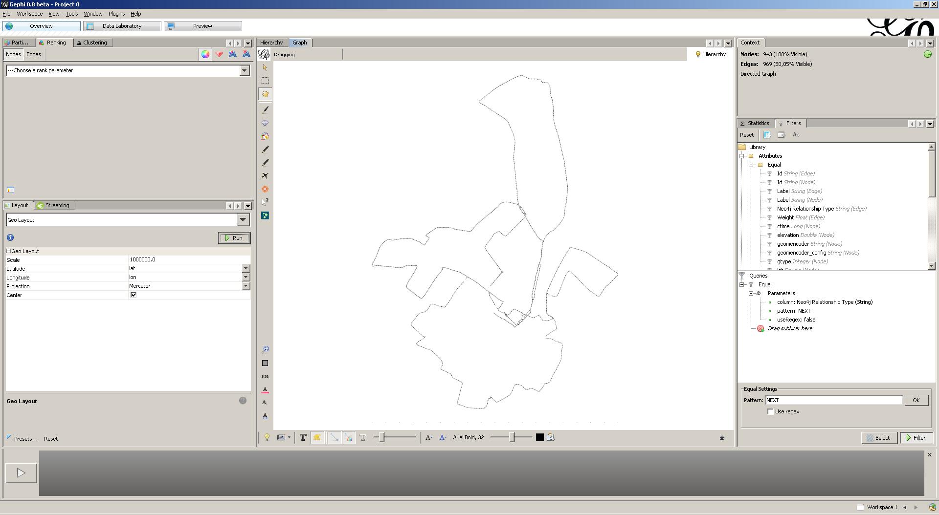
Only half of the edges remain … However, we will still not gain novel insights from this mess. Let’s layout our graph by using the Gephi GeoLayout plugin. This layouter takes geocoded graphs as input and will layout graphs according to the geocoded attributes. Make sure to increase scaling, as our coordinates are located closely together. Cool! This view clearly outlines the courses I’m running.
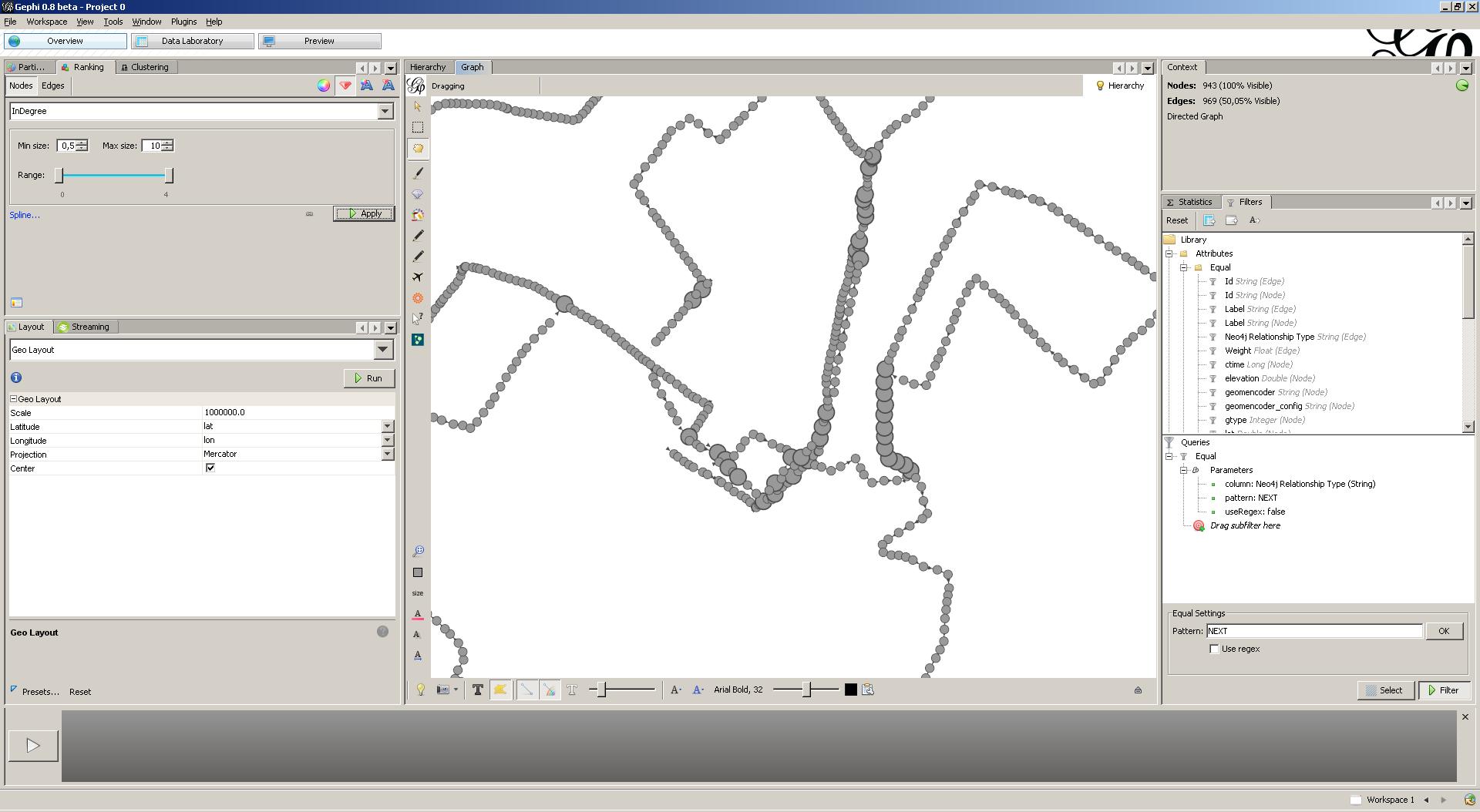
Let’s visualize the coordinates that were frequently encountered during the 4 runs that are imported in the Neo4J Spatial datastore. For this, we will use the InDegree node property, which indicates the number of incoming edges for each coordinate. We rank node weight (i.e. node size) through this property. Hence, frequently encountered nodes will show up bigger. In my case, frequently encountered coordinates are found around the place where I live (and hence start my runs) and on street intersections.
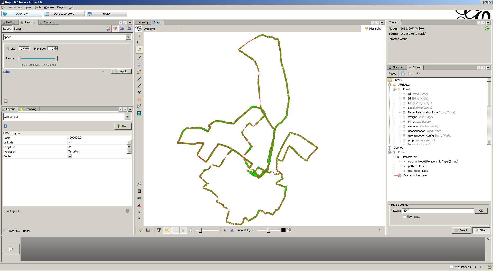
Let’s do one final analysis, namely a visualization that illustrates the average pace throughout all runs. For this, we rank both node weight and node color through the speed property. Hence, coordinates with a high average pace are colored green and show up bigger. Coordinates with a low average pace are colored red and show up smaller. With the blink of an eye, I can now interpret my average pace, taking into account my overall running data set!
4. Conclusion
This article describes the use of the Neo4J Spatial datastore and Gephi to analyze Garmin running data. As always, the complete source code can be found on the Datablend public GitHub repository. Any ideas for other types of analysis that could be performed on the dataset?